iPhone Videos are missing audio when imported to Premiere Pro - fix options

So we shot some video today using the iPhone X and the app Hylerlapse, but when I tried bringing the video file into Premiere Pro CC 2018, the audio isn't there.

A quick perusal of the web yielded the most popular solutions.  These options showed promise but they didn't work for me.  Maybe they would work for your situation.

Tricks that didn't work for me:

1.  Select "New Sequence from Clip" in Premiere Pro (like this guy says to do)

2.  Change the file extension from .mov to .mp3 by renaming the file, then import it (like this guy says will work)

So for me, the only solution that does work is to convert the .mov file to an .mp4 using a conversion tool.  For some reason I can't do this with Adobe Media Encoder, go figure, so I looked for a few alternatives.

There are a lot of video conversion tools out there, but the one that I chose is Wondershare Uniconverter.  It cost me real money, $70 for a lifetime license, so this is a solution for the individual that plans on doing this repeatedly.  

Here's the Link:  https://videoconverter.wondershare.com/

One weird thing to note, Uniconverter didn't recognize the orientation from the phone video, so my stuff showed up upside-down.  That's okay because I'm taking these into Premiere Pro to lighten the vids up and rotation is super easy to do, but it did catch me off-guard when I saw this the first time.

Excel: Quick way to check if a cell begins with a value

For this exercise, I wanted to make a pivot table to help me summarize my orders by product type.  I had a single column with the Product Name, but sometimes a product is included in a bundle so I wanted to create a column for each product and put a 1 or a 0 in the column if that item was included in that sale bundle.  

Let's same the product names are:
Creative Lettering Journal
The Guide to Mindful Lettering
Ultimate Lettering Bundle (This has both the Lettering Journal and the Guide)

Since the first three letters of each product are distinct I can use those to differentiate each.  Assume the Product Name is in Column A.  In the column where I'm tallying the Creative Lettering Journals I use the following formula:

formula =IF(Left(A2,3)="Cre",1,if(Left(A2,3)="Ult",1,0))

Now I have a single column that tells me exactly how many Creative Lettering Journals were sold.

Excel: Remove extra spaces from a cell

I found this tutorial on using TRIM and SUBSTITUTE to remove spaces from a cell very useful:

http://www.pryor.com/blog/remove-extra-spaces-from-excel-data/

Excel: Create an Option List in a cell

Here's how to create an option set for a cell in Excel 2016.

So I have a form I'm creating and I want to limit the optional values in one column.  Here's a simple description of what I'm putting together.

The Column Name is "Status".  I want to make a limit the options for this cell instead of having it be filled in with any number of values.  If I can get consist data entry in this field I can then use it to filter the table or to pivot the data for further analysis.

Here are the options I want to make available:

• Potential Buy
• New Purchase
• In Rehab
• Listed
• Pending
• Sold

So, here's the step by step.

1. Create the options list on a separate page from your working doc

2. Select the cells that you want to use the option list

3. Go to the Data menu and click Validation

4. In the Validation Window select "List" from the Allow menu
5. Click the Source box and select the cells that show the options you want to use

1. Create the options list on a separate page from your working doc

2. Select the cells that you want to use the option list

3. Go to the Data menu and click Validation

4. In the Validation Window select "List" from the Allow menu

5. Click the Source box and select the cells that show the options you want to use

6.  The Option List should now be available for your cells

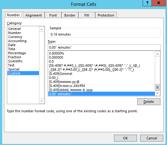
Excel: Change a cell format to add text after a Number

Microsoft: Create a Custom Number Format

From Microsoft:
Display both text and numbers    To display both text and numbers in a cell, enclose the text characters in double quotation marks (" ") or precede a single character with a backslash (\). Include the characters in the appropriate section of the format codes. For example, type the format $0.00" Surplus";$-0.00" Shortage" to display a positive amount as "$125.74 Surplus" and a negative amount as "$-125.74 Shortage." Note that there is one space character before both "Surplus" and "Shortage" in each code section.

So I selected format Category "Custom", then in the Type field I typed " minutes" right after the 0.00.  That did the trick!

Excel - Mortgage Principal Paid over a Period

Interested in determining how much principal is paid on a mortgage between two time periods?


CUMPRINC(Rate, nper, pv, start_period, end_period, type)

Example: How much principal will a borrower pay between their 10 and 15 payment on their mortgage?  Principal balance at the starting period is $51000 and interest rate in 9%.

Rate - it's the interest rate for the period, so for a mortgage with 9% you need to divide by 12 to get the monthly interest rate, .09/12

nper - total number of payments to be included, so the number of months between the start period and end period  (15-10), 5

pv - the principal at the starting period

Start_Period - Payment date doesn't work, you have to figure out the payment number, i.e. the 10th payment out of the term. 10

End_Period - Again, not a date, it has to be the number of the last payment, 15

Type - set it to 0 if the payment is made on the first of the month, 1 of the payment is on the end of the month

=CumPrinc( .09/12, 5, 51000, 10, 15)

Cumulative Principal Paid Between Periods

Excel - Countifs Using Equal To or Greater Than with a Date Field

There's a wrinkle in the countifs() formula for using a date field rather than an explicitly declared date in the formula.

Here's an example:
=COUNTIFS($P$15:$P$2050,"91+",$D$15:$D$2050,$A$1,$Q$15:$Q$2050,">=1/10/2013")

I wanted to replace the "1/10/2013" with a date field in A3.

My first attempt was this:
=COUNTIFS($P$15:$P$2050,"91+",$D$15:$D$2050,$A$1,$Q$15:$Q$2050,">=$A$3")
Which doesn't work.  My next try was this:

=COUNTIFS($P$15:$P$2050,"91+",$D$15:$D$2050,$A$1,$Q$15:$Q$2050,">="$A$3)
Again, that didn't work.


Now here's the correct way to use a date field in Countifs():

=COUNTIFS($P$15:$P$2050,"91+",$D$15:$D$2050,$A$1,$Q$15:$Q$2050,">="&$A$3)

See that little ampersand between the greater than and equal section and the field?  That's the trick.


You're welcome.