For this exercise, I wanted to make a pivot table to help me summarize my orders by product type. I had a single column with the Product Name, but sometimes a product is included in a bundle so I wanted to create a column for each product and put a 1 or a 0 in the column if that item was included in that sale bundle.
Let's same the product names are:
Creative Lettering Journal
The Guide to Mindful Lettering
Ultimate Lettering Bundle (This has both the Lettering Journal and the Guide)
Since the first three letters of each product are distinct I can use those to differentiate each. Assume the Product Name is in Column A. In the column where I'm tallying the Creative Lettering Journals I use the following formula:
formula =IF(Left(A2,3)="Cre",1,if(Left(A2,3)="Ult",1,0))
Now I have a single column that tells me exactly how many Creative Lettering Journals were sold.
Tuesday, January 2, 2018

Monday, August 21, 2017
Excel: Remove extra spaces from a cell
I found this tutorial on using TRIM and SUBSTITUTE to remove spaces from a cell very useful:
http://www.pryor.com/blog/remove-extra-spaces-from-excel-data/
http://www.pryor.com/blog/remove-extra-spaces-from-excel-data/
Monday, December 12, 2016
Excel: Create an Option List in a cell
Here's how to create an option set for a cell in Excel 2016.
So I have a form I'm creating and I want to limit the optional values in one column. Here's a simple description of what I'm putting together.
The Column Name is "Status". I want to make a limit the options for this cell instead of having it be filled in with any number of values. If I can get consist data entry in this field I can then use it to filter the table or to pivot the data for further analysis.
Here are the options I want to make available:

So I have a form I'm creating and I want to limit the optional values in one column. Here's a simple description of what I'm putting together.
The Column Name is "Status". I want to make a limit the options for this cell instead of having it be filled in with any number of values. If I can get consist data entry in this field I can then use it to filter the table or to pivot the data for further analysis.
Here are the options I want to make available:
- Potential Buy
- New Purchase
- In Rehab
- Listed
- Pending
- Sold
So, here's the step by step.
1. Create the options list on a separate page from your working doc
2. Select the cells that you want to use the option list
3. Go to the Data menu and click Validation
4. In the Validation Window select "List" from the Allow menu
5. Click the Source box and select the cells that show the options you want to use

2. Select the cells that you want to use the option list

5. Click the Source box and select the cells that show the options you want to use
1. Create the options list on a separate page from your working doc

2. Select the cells that you want to use the option list

3. Go to the Data menu and click Validation

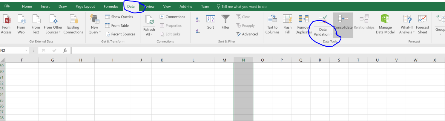
4. In the Validation Window select "List" from the Allow menu

5. Click the Source box and select the cells that show the options you want to use

6. The Option List should now be available for your cells


5. Click the Source box and select the cells that show the options you want to use

6. The Option List should now be available for your cells

Monday, April 27, 2015
Excel: Change a cell format to add text after a Number
Microsoft: Create a Custom Number Format
From Microsoft:
Display both text and numbers To display both text and numbers in a cell, enclose the text characters in double quotation marks (" ") or precede a single character with a backslash (\). Include the characters in the appropriate section of the format codes. For example, type the format $0.00" Surplus";$-0.00" Shortage" to display a positive amount as "$125.74 Surplus" and a negative amount as "$-125.74 Shortage." Note that there is one space character before both "Surplus" and "Shortage" in each code section.
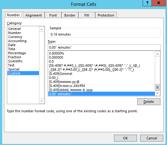
So I selected format Category "Custom", then in the Type field I typed " minutes" right after the 0.00. That did the trick!
From Microsoft:
Display both text and numbers To display both text and numbers in a cell, enclose the text characters in double quotation marks (" ") or precede a single character with a backslash (\). Include the characters in the appropriate section of the format codes. For example, type the format $0.00" Surplus";$-0.00" Shortage" to display a positive amount as "$125.74 Surplus" and a negative amount as "$-125.74 Shortage." Note that there is one space character before both "Surplus" and "Shortage" in each code section.
So I selected format Category "Custom", then in the Type field I typed " minutes" right after the 0.00. That did the trick!
Tuesday, February 4, 2014
Excel - Mortgage Principal Paid over a Period
Interested in determining how much principal is paid on a mortgage between two time periods?
CUMPRINC(Rate, nper, pv, start_period, end_period, type)
Example: How much principal will a borrower pay between their 10 and 15 payment on their mortgage? Principal balance at the starting period is $51000 and interest rate in 9%.
Rate - it's the interest rate for the period, so for a mortgage with 9% you need to divide by 12 to get the monthly interest rate, .09/12
nper - total number of payments to be included, so the number of months between the start period and end period (15-10), 5
pv - the principal at the starting period
Start_Period - Payment date doesn't work, you have to figure out the payment number, i.e. the 10th payment out of the term. 10
End_Period - Again, not a date, it has to be the number of the last payment, 15
Type - set it to 0 if the payment is made on the first of the month, 1 of the payment is on the end of the month
=CumPrinc( .09/12, 5, 51000, 10, 15)
Cumulative Principal Paid Between Periods
Thursday, January 16, 2014
Excel - Countifs Using Equal To or Greater Than with a Date Field
There's a wrinkle in the countifs() formula for using a date field rather than an explicitly declared date in the formula.
Here's an example:
=COUNTIFS($P$15:$P$2050,"91+",$D$15:$D$2050,$A$1,$Q$15:$Q$2050,">=1/10/2013")
I wanted to replace the "1/10/2013" with a date field in A3.
My first attempt was this:
=COUNTIFS($P$15:$P$2050,"91+",$D$15:$D$2050,$A$1,$Q$15:$Q$2050,">=$A$3")
Which doesn't work. My next try was this:
=COUNTIFS($P$15:$P$2050,"91+",$D$15:$D$2050,$A$1,$Q$15:$Q$2050,">="$A$3)
Again, that didn't work.
Now here's the correct way to use a date field in Countifs():
=COUNTIFS($P$15:$P$2050,"91+",$D$15:$D$2050,$A$1,$Q$15:$Q$2050,">="&$A$3)
See that little ampersand between the greater than and equal section and the field? That's the trick.
You're welcome.
Here's an example:
=COUNTIFS($P$15:$P$2050,"91+",$D$15:$D$2050,$A$1,$Q$15:$Q$2050,">=1/10/2013")
I wanted to replace the "1/10/2013" with a date field in A3.
My first attempt was this:
=COUNTIFS($P$15:$P$2050,"91+",$D$15:$D$2050,$A$1,$Q$15:$Q$2050,">=$A$3")
Which doesn't work. My next try was this:
Again, that didn't work.
Now here's the correct way to use a date field in Countifs():
=COUNTIFS($P$15:$P$2050,"91+",$D$15:$D$2050,$A$1,$Q$15:$Q$2050,">="&$A$3)
See that little ampersand between the greater than and equal section and the field? That's the trick.
You're welcome.
Thursday, November 7, 2013
Excel - Grouping Dates by Month in a Pivot Table
For this post I am referencing the work creating by the talented minds at Chandoo.org, a great resource for advancing your knowledge of Excel. Here's the direct link to their pivot table post.
I ran into a problem when creating a pivot table yesterday. Here's my raw data, a series of daily bank payments that I wanted to group to show what months the account had made payments in.

Creating the pivot is pretty easy, but the result is that for each account the payments show up by day instead of summed up by month.

Here's the trick that the guys at Chandoo.org showed me. Right click on a date cell; the pull-down menu will show a category called "Group...". Click Group and you can select month, year, etc.
The result is a nice pivot table with your numbers summed up by month.

One caveat, it seems when you group by month it only looks at the month part of a date field, so if you have dates spanning multiple years they will get summed up to the specific month. So you have to select group by month and year, this will do the trick!
I ran into a problem when creating a pivot table yesterday. Here's my raw data, a series of daily bank payments that I wanted to group to show what months the account had made payments in.

Creating the pivot is pretty easy, but the result is that for each account the payments show up by day instead of summed up by month.

Here's the trick that the guys at Chandoo.org showed me. Right click on a date cell; the pull-down menu will show a category called "Group...". Click Group and you can select month, year, etc.


The result is a nice pivot table with your numbers summed up by month.
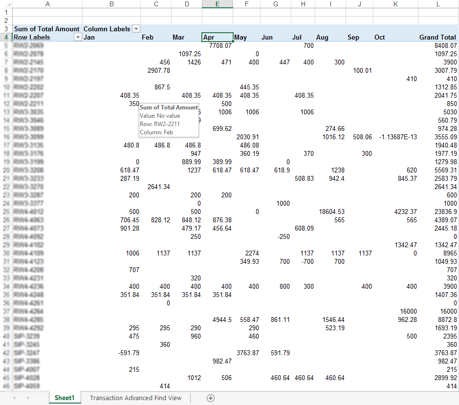
One caveat, it seems when you group by month it only looks at the month part of a date field, so if you have dates spanning multiple years they will get summed up to the specific month. So you have to select group by month and year, this will do the trick!
Subscribe to:
Posts (Atom)